Learning Objective: In this tutorial, you are going to learn how to create a SQL Server Indexed view that stored data physically in the database.
Introduction to the SQL Server indexed view
Views provide a way to represent the table data in a more effective manner by implementing simplicity, business logic, and row and column level security. They do not store any data within themselves. They fetch the data from the underlying tables mentioned in the views. However, views are not meant for performance improvement.
Unlike regular view, indexed view are the materialized view where they store the data physically to improve the performance of the query if they are properly used.
In order to create a view, you use the following steps:
First, create a view using WITH SCHEMABINDING option which binds the view to the schema of the underlying tables.
Second, create a unique clustered index on the view. This materializes the view.
Because of the WITH SCHEMABINDING option, if you want to change the structure of the underlying tables, you must drop the indexed view first before applying the changes.
In addition to the above, SQL Server requires all the object references in an indexed view to include a two-part naming convention i.e. schema.object, all the referenced objects are in the same database.
Whenever the data of the underlying tables changes, the data in the indexed view also automatically updated. This result writes overhead for the referenced tables. It means that when you insert any records in the underlying tables, SQL Server also has to write the data into the indexed view. Therefore, it is recommended to use the indexed table only when the data of the table is updated infrequently.
Creating an SQL Server indexed view example
Let’s consider below two tables in SQL Server Database,
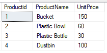
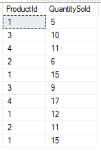
Script to create above tables
create table tblProduct (
 Productid int PRIMARY KEY,
 ProductName varchar(20),
 UnitPrice int
 );
 insert into tblProduct values (1,'Bucket',150);
 insert into tblProduct values (2,'Plastic Bowl',60);
 insert into tblProduct values (3,'Plastic Bottle',30);
 insert into tblProduct values (4,'Dustbin',100);

Create Table tblProductSales
 (
  ProductId int,
  QuantitySold int
 );
 Insert into tblProductSales values(1, 5);
 Insert into tblProductSales values(3, 10);
 Insert into tblProductSales values(4, 11);
 Insert into tblProductSales values(2, 6);
 Insert into tblProductSales values(1, 15);
 Insert into tblProductSales values(3, 9);
 Insert into tblProductSales values(4, 17);
 Insert into tblProductSales values(1, 12);
 Insert into tblProductSales values(2, 11);
 Insert into tblProductSales values(1, 15);
Now create a view to get the Total Sales by ProductName.
Create view vWTotalSalesByProduct
 with SCHEMABINDING
 as
 Select ProductName,
 SUM(ISNULL((QuantitySold * UnitPrice), 0)) as TotalSales,
 COUNT_BIG(*) as TotalTransactions
 from dbo.tblProductSales
 join dbo.tblProduct
 on dbo.tblProduct.ProductId = dbo.tblProductSales.ProductId
 group by ProductName;
Notice the WITH SCHEMABINDING option after the view name. The rest is the same as the regular view.
Before creating a unique clustered index for the view, let’s examine the query I/O cost statistics by querying data from a regular view and using the SET STATISTICS IO command:
SET STATISTICS IO ON
 GO
 SELECT
     *
 FROM
     dbo.vWTotalSalesByProduct
 ORDER BY
     ProductName;
 GO
SQL Server returns the following query I/O cost statistics:
Table 'tblProductSales'. Scan count 1, logical reads 4, physical reads 0, page server reads 0, read-ahead reads 0, page server read-ahead reads 0, lob logical reads 0, lob physical reads 0, lob page server reads 0, lob read-ahead reads 0, lob page server read-ahead reads 0.
 Table 'Worktable'. Scan count 0, logical reads 0, physical reads 0, page server reads 0, read-ahead reads 0, page server read-ahead reads 0, lob logical reads 0, lob physical reads 0, lob page server reads 0, lob read-ahead reads 0, lob page server read-ahead reads 0.
 Table 'tblProduct'. Scan count 1, logical reads 2, physical reads 0, page server reads 0, read-ahead reads 0, page server read-ahead reads 0, lob logical reads 0, lob physical reads 0, lob page server reads 0, lob read-ahead reads 0, lob page server read-ahead reads 0.
As you can see clearly from the output, SQL Server had to read from three corresponding tables before returning the result set.
Now let’s create a unique cluster index to the view.
This statement makes the view dbo.vWTotalSalesByProduct as materialized view which has the physical existence in the database.
You can also add a non-clustered index on the ProductName column of the view:
CREATE UNIQUE CLUSTERED INDEX
     UIX_vWTotalSalesByProduct_ProductName
 ON dbo.vWTotalSalesByProduct(ProductName);
Now, if you query data against the view, you will notice that the statistics have changed:
Table 'vWTotalSalesByProduct'. Scan count 1, logical reads 2, physical reads 0, page server reads 0, read-ahead reads 0, page server read-ahead reads 0, lob logical reads 0, lob physical reads 0, lob page server reads 0, lob read-ahead reads 0, lob page server read-ahead reads 0.
Here, SQL Server instead of reading from the three different tables reads the data from the materialized view product_master directly which improved the performance of the query.
Summary: In this tutorial, you have learned how to create an indexed view and use them to improve the performance of the query in the SQL Server database.